QEFs, Eigenvalues, and Normals
Given a distance field and a spatial region that contains a zero crossing (i.e. an inside-to-outside transition), there's a neat strategy for placing a vertex at a useful position.
This post explains this strategy, but only as a prelude: the novel bit is at the end, where I discuss how to use this strategy to also pick out characteristic normals at that vertex.
Intuition
Let's say you've found a bunch of zero crossings of a distance field, and can evaluate the normals at each point (either numerically or with automatic differentiation).
For example, here's the distance field describes a rotated rectangle corner:
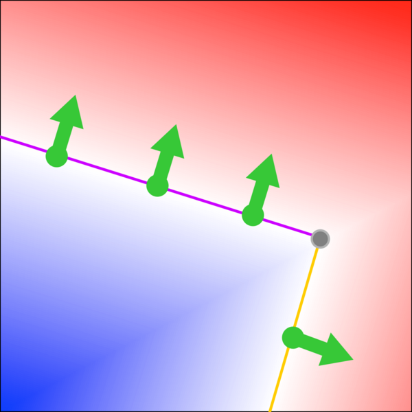
Inside vs. outside is indicated with blue vs. red shading; the zero crossings and their normals are drawn as green points and arrows.
Each of these position + normal points implies a edge, which touches the point and is orthogonal to the normal. In the figure above, the top three points imply the purple edge, and the bottom point implies the yellow edge.
We want to solve for a point that is on every edge, or a close as possible. In our 2D example, it's simply the rectangle's corner (drawn in grey).
Matrix math
Let's begin to formalize our intuitive understanding.
We'll name the zero crossings $ (p_1, n_1), (p_2, n_2), (p_3, n_3), ... $.
If we're trying to solve for a vertex position $ x$, then we want the projection of $n_i$ onto $x - p_i$ to be zero for all $i$. This is the "point on every edge" criterion that we described above.
We'll construct an error function that measures how close we are to meeting this goal, using a quadratic form for reasons that will become clear shortly:
$$ E(x) = \sum \left( n_i \cdot \left( x - p_i \right) \right) ^2 $$
The ideal value for $x$ is one that minimizes this error function, ideally driving it to zero.
Now, let's begin shuffling around symbols to put things into a different form. We can reframe the array of dot products as a matrix multiplication, introducing an intermediate function $D(x)$:
$$ D(x) = \left[ \begin{array}{c} n_1 \\ n_2 \\ ... \end{array} \right ] \left( x - \left[ \begin{array}{ccc} p_1 & p_2 & ... \end{array} \right ] \right)$$
where every $n_i$ is a row vector, and every $p_i$ and $x$ are column vectors; $ D(x) $ is then a column vector with as many items as there are intersection points.
The error function can be expressed as $ E(x) = D(x)^T D(x) $, which performs the sum-of-squares operation.
Now, let's expand $ D(x) $: $$ D(x) = \left[ \begin{array}{c} n_1 \\ n_2 \\ ... \end{array} \right ] x - \left[ \begin{array}{c} n_1 \\ n_2 \\ ... \end{array} \right ] \left[ \begin{array}{ccc} p_1 & p_2 & ... \end{array} \right ] $$
We'll define two new matrices, $ A $ and $ b $:
$$ A = \left[ \begin{array}{c} n_1 \\ n_2 \\ ... \end{array} \right] $$
$$ b = \left[ \begin{array}{c} n_1 \cdot p_1 \\ n_2 \cdot p_2 \\ ... \end{array} \right] $$
Now, we have $ D(x) = Ax - b $ and $ E(x) = \left( Ax - b \right) ^T \left( Ax - b \right) $
Solving for $ x $ can now be done by solving the least-squares problem $ Ax = b $.
Neat!
Compact representation
Dual Contouring (linked below) introduces a more space-efficient strategy for doing this computation: instead of storing $ A $ and $ b $, they observed the expanded error function is of the form
$$ E(x) = x^TA^TAx + 2x^TA^Tb + b^Tb $$
You can store $ A^TA $, $A^Tb $, and $ b^Tb $, as a compact representation for the QEF.
Solving the QEF from this form is documented in the "Secret Sauce" paper linked below. I won't copy all the math over, but know that it involves solving for the eigenvectors and eigenvalues of $ A^T A $.
One weird eigenvalues trick
For rendering reasons, I'm interested in extracting the characteristic normals from the QEF. For example, let's say we've found a bunch of intersections in 3D space with normals that look like this:
A = array([[ 0.      ,  0.      , -1.      ],
           [-0.707107, -0.707106,  0.      ],
           [-0.707107, -0.707106,  0.      ],
           [-0.707107, -0.707106,  0.      ],
           [-0.707106,  0.707107,  0.      ],
           [-0.707106,  0.707107,  0.      ],
           [ 0.      ,  0.      , -1.      ],
           [-0.707106,  0.707107,  0.      ]])
(this is the $ A $ matrix discussed above)
I'd like to start from this matrix and extract out
   [[ 0.      ,  0.      , -1.],
    [-0.707107, -0.707106,  0.],
    [-0.707106,  0.707107,  0.]]
as the three characteristic normals.
This matrix multiplication $ A^T A $ looks suspicious like a step in computing the principle components of the matrix $ A $. That sounds promising!
The next step in that PCA recipe is to find the eigenvalues of this matrix – which we already needed to do, to find the vertex – so maybe we'll get the characteristic normals for free:
>>> np.linalg.eig(A.T.dot(A))[1]
array([[ 1.,  0.,  0.],
       [ 0.,  1.,  0.],
       [ 0.,  0.,  1.]])
Nope.
This is where I got stuck for a few days. The characteristic normals are right there in the matrix, but I couldn't figure out how to convince an eigenvector solver to pick them out.
Finally, I figured out the issue: In that matrix, all of the normals have the same length, so one orthogonal basis is as good as the next.
However, if we tweak the lengths, then we can force the eigenvalues to line up with the characteristic normals:
>>> A_ = A * np.vstack([np.arange(A.shape[0]) + 1] * 3).T
>>> A_
array([[ 0.      ,  0.      , -1.      ],
       [-1.414214, -1.414212,  0.      ],
       [-2.121321, -2.121318,  0.      ],
       [-2.828428, -2.828424,  0.      ],
       [-3.53553 ,  3.535535,  0.      ],
       [-4.242636,  4.242642,  0.      ],
       [ 0.      ,  0.      , -7.      ],
       [-5.656848,  5.656856,  0.      ]])
>>> np.linalg.eig(A_.T.dot(A_))[1]
array([[-0.70710728,  0.70710628,  0.        ],
       [-0.70710628, -0.70710728,  0.        ],
       [ 0.        ,  0.        ,  1.        ]])
This one weird trick forces the eigenvectors to represent the main normals in the $ A $ matrix!
There are only two caveats:
- The eigenvectors / normals may be inverted.
- You'll also need to scale the other matrices when solving for vertex position.
Still, this is a neat way to extract normals (basically for free) from a QEF-based vertex position calculation.
If you're one of the three other people on earth that this is useful for, feel free to send me an email
References
The original quadratic error metrics paper.
The two papers that helped me understand the technique are Feature Sensitive Surface Extraction from Volume Data and the famous Dual Contouring of Hermite Data (along with its companion Dual Contouring: "The Secret Sauce").